Dominator Tree of a Directed Graph

Link to pdf version.

Introduction : In this article I am going to explain the concept of Dominators in a directed graph, its applications and an efficient algorithm for construction of dominator tree published by Robert Tarjan [1].

Since there is a lot of content to be covered, the post is going to be a bit long. So, please be patient. 🙂

Pr-requisites : dfs in directed graphs. DSU

Basic Definitions

• Dominator : Dominators are defined in a directed graph with respect to a source vertex S. Formally, A node u is said to dominate a node w wrt source vertex S if all the paths from S to w in the graph must pass through node u.
  Note that only the vertices that are reachable from source vertex in the directed graph are considered here. Hence, Hereafter in the article it is assumed that every vertex in the graph is reachable from the source.
• Immediate Dominator : A node u is said to be an immediate dominator of a node w (denoted as idom(w)) if u dominates w and every other dominator of w dominates u.

Theorem-1: Every vertex of the directed graph, except the source S,will have at-least one dominator.
Proof : Since every path from source S to any vertex w in the graph always passes through the source vertex, hence the source vertex S dominates every other vertex in the graph.

Theorem-2: Every vertex of the directed graph, except the source S, has a unique idom.
Proof : Let u and v be two idoms of a vertex w ( S) . By definition of idom, u should dominate v and v should dominate u but since dominator relationship is anti-symmetric, it leads to a contradiction!

• Dominator Tree :  The edges forms a directed tree with S being the root r of the tree.
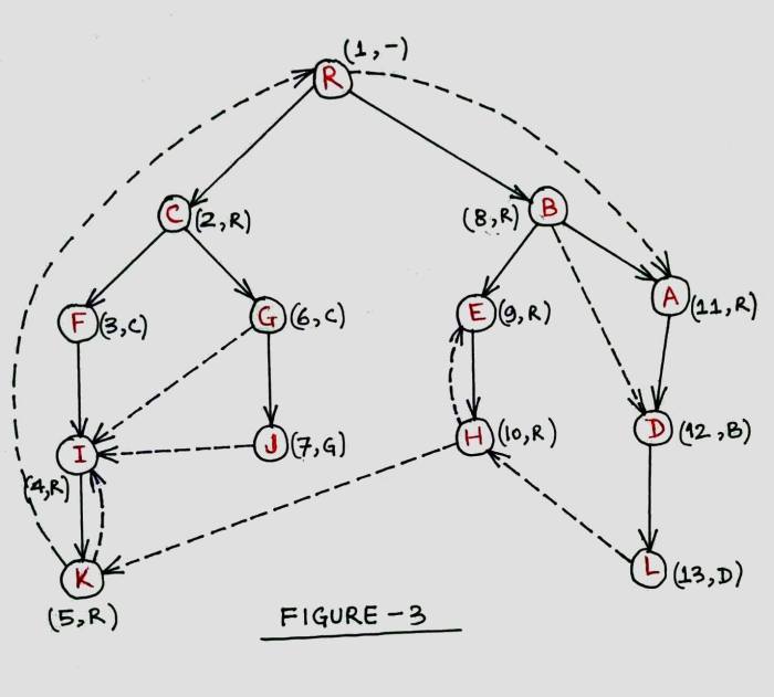
  Fig1 shows a directed graph with the source vertex marked and Fig2 shows it’s corresponding dominator tree wrt the source vertex. Before proceeding further, try to come up with an algorithm (irrespective of the complexity) to build the dominator tree of a given graph.

A naive O(N*M) approach :

A naive approach to build the dominator tree could be that initially  do a dfs from the source vertex to check what all vertices are reachable from the source. Then, for each vertex w , remove the vertex from the graph and again do dfs from source vertex and all those vertices which were earlier visited but not now are the ones that are dominated by vertex w. Once we do this for every vertex of the graph, for every vertex we shall have a list of all the vertices that this vertex dominates i.e. a list of all the vertices that lie in the subtree of this vertex in the dominator tree. Hence, we can easily construct the dominator tree using this information. Since we perform one dfs for every vertex in the graph, complexity would be O(n*m).

A Faster O((n+m)logN) approach :

Before explaining the faster approach,

• We do a dfs on the given graph from the source vertex and assign new numbers to each vertex of the graph which would be equal to the arrival time of the vertex in the spanning tree T obtained by the dfs.
• Also, we define another term called semi-dominator (written as sdom)  as:

The following graph shows semi-dominators marked for every vertex of the graph given in Fig-1.

A few important points regarding semi-dominators:

1. If w S be any vertex , then sdom(w) is a proper ancestor of w in the dfs tree T.
   Proof : By definition of sdom, parent(w) in the spanning tree T is one of the candidates for sdom. Hence, sdom(w)<=parent(w). Now let sdom(w)  not be an ancestor of w. Then, sdom(w) would lie in a subtree towards the left side of w. Now in such a case, there should exist a non-tree edge coming from a left subtree towards the right subtree to satisfy the definition of sdom, which is not possible. Hence sdom(w) will always be an ancestor of w.
2. If w S be any vertex, then idom(w) is an ancestor (not necessarily proper) of sdom(w) in the dfs tree T.
   Proof : Clearly, idom(w) must lie on the path from source to w in the spanning tree T because if it is not, there would be a path from source to w not passing through idom(w) which leads to a contradiction! Also, by definition of sdom, idom(w) cannot lie on the path from sdom(w) to w in the spanning tree T. Hence, idom(w) is an ancestor of sdom(w).
3. Let v be an ancestor of w  in the spanning tree T, then either
   ->v is an ancestor of idom(w) or
   ->idom(w) is an ancestor of idom(v)
   Proof : Let idom(w) be an ancestor of v and idom(v) be an ancestor of idom(w), then there exist a path from idom(v) to v avoiding idom(w) in the graph. Also, since v is an ancestor of w, it implies that there exists a path from idom(v) to w avoiding idom(w). This leads to a contradiction! Hence, either v is ancestor of idom(w) or idom(w) is an ancestor of idom(v).
4. Let w S. If, for every vertex u which is an ancestor of w and has sdom(w) as its proper ancestor, sdom(u) >= sdom(w) then idom(w)=sdom(w).
   Proof : Let idom(w) be a proper ancestor of sdom(w). It implies that there exists a path from idom(w) to w avoiding sdom(w) in the graph. Now there are 2 different ways this path could exist :
   • The path avoids all the nodes from w to sdom(w) in the spanning tree (see fig below). In such a case sdom(w) would have been higher in the tree (as marked in the fig.). This leads us to a contradiction!
     
   • The path avoids sdom(w) and includes some other vertex v from w to sdom(w) (see fig below). In such a case, sdom(v) < sdom(w) which is not possible. This also leads us to a contradiction!
     
5. Let w S. Let u be a vertex for which sdom(u) is minimum among all vertices u satisfying “sdom(w) is a proper ancestor of u and u is an ancestor of w”.  If sdom(u)<=sdom(w) then idom(w) = idom(u).
   Proof : Clearly, idom(w) <= idom(u) by point 3 (above). Let idom(w) < idom(u). There must exist a path from idom(w) to w avoiding idom(u). Now there could be 2 different ways this path could exist :
   • The path avoids all the nodes from w to sdom(w) in the spanning tree . In such a case sdom(w) would have been higher in the tree. Very similar reasoning like point 4.
   • Let y be the first node on the path from idom(w) to w such that idom(u) is an ancestor of y and y is an ancestor of w. y can either lie above u or below u .
     • If y lies above u (see Fig 6 below) , there would be a path from idom(w) to u avoiding idom(u) which leads to a contradiction.
     • If y lies below u (see Fig 6 below) , sdom(y) < sdom(u) which is not possible because u was the node with min sdom among all the nodes between w and sdom(w). Again, this leads to a contradiction.
       
   • Hence, y=idom(w)=idom(u) is the only possibility. Hence idom(u) dominates w.
6. Let w S. Let u be a vertex for which sdom(u) is minimum among all vertices u satisfying “sdom(w) is a proper ancestor of u and u is an ancestor of w”.  Then :

   

   Proof : Follows directly form points 4 and 5 above.

How to calculate sdom ?

Now given the above properties of sdom, idom for every vertex can be easily calculated given that we have already computed sdoms. The following theorem provides a way to compute sdoms :

      

In simple words, sdom(w) is the minimum node lying in the union of following two groups :  (remember labels of nodes correspond to the arrival times in dfs tree !) :

• All the nodes v such that (v,w) is a directed edge in the graph and v < w. That is, all the ancestors of w that have a forward edge from itself to w.
• sdom(u) where u > w and there is an edge (v,w) in the graph such that u is an ancestor of v. What that really means is that for all nodes u > w (u can either be in the subtree of w (see Fig 7) or in the subtrees towards right of w (see Fig 7)) if u is an ancestor of any node node v such that (v,w) is an edge, then consider sdom(u) for sdom(w). This is important because since u>w and u is an ancestor of a node v such that (v,w) is an edge , if we can reach u by any path then the path from u to w doesn’t include any node < w. I have tried to provide a basic intuition here. For a more concrete proof, refer the original research paper mentioned below in references.
  

Faster Algorithm For Building Dominator Tree

The steps of the algorithm are as follows :

Step-1: Carry out a dfs on the input graph and assign new labels to the vertices , equal to the arrival time of the vertex in the dfs. Also initialize other variables used in the implementation.
The following variables are used in the implementation of the algorithm (see further points for a better understanding of each variable) :

VI g[N],tree[N],rg[N],bucket[N];
int sdom[N],par[N],dom[N],dsu[N],label[N];
int arr[N],rev[N],T;
//1-Based directed graph input

• g[N] : input graph. rg[N] : reverse graph. tree[N] : final dominator tree.
• arr[N] : mapping of i’th node to its new index, equal to the arrival time of node in dfs tree. par[N] : parent of node i in dfs tree. rev[N] : reverse mapping of i’th node to the original label in input graph.
• sdom[N] : label of semi-dominator of the i’th node. Initially sdom[i]=i.
• dom[N] : label of immediate-dominator of the i’th node. Initially dom[i]=i.
• bucket[N] : For a vertex i, it stores a list of vertices for which i is the semi-dominator. Initially it is empty.
• dsu[N] : parent of i’th node in the forest maintained during step 2 of the algorithm. Initially dsu[i] = i.
• label[N] : At any point of time, label[i] stores the vertex v with minimum sdom, lying on path from i to the root of the (dsu) tree in which node i lies. Initially, label[i]=i. The implementation of this step is as follows :

void dfs0(int u)
{
	T++;arr[u]=T;rev[T]=u;
	label[T]=T;sdom[T]=T;dsu[T]=T;
	for(int i=0;i<SZ(g[u]);i++)
	{
		int w = g[u][i];
		if(!arr[w])
		{
			dfs0(w);
			par[arr[w]]=arr[u];
		}
		rg[arr[w]].PB(arr[u]);
	}
}

---

Step-2: Compute semi-dominator of all vertices by applying the theorem mentioned in previous section. Carry out the computation vertex by vertex in decreasing order by number.

This is the most important step of the algorithm. For any vertex w in the graph, there could be 4 different types of in-edges (tree edge,back edge,forward edge and cross-edge) for w in the spanning tree formed by dfs (Refer figure in previous section).

Now, we shall process the vertices in decreasing order of number and maintain a forest of all the vertices that have already been processed. Once a vertex is processed , the value of its sdom would have been calculated. Also, to maintain the forest of processed vertices we use dsu data structure that should support the following operations :

• Find(v): Let r be the root of (dsu) tree in which node v lies.
  • If v==r, return v .
  • else return a node u(!=r) with minimum sdom , lying on path from v to r.
• Union(u,v): Merge the (dsu) trees in which u and v lies.

Implementation of the above two functions is discussed later.

Now, to process a node w and calculate its sdom we look at all the incoming edges of node w. Let (v,w) be an incoming edge, then

• If v < w i.e. v is an ancestor of w, v would not have been processed till now and hence Find(v) would return v.
• If v > w i.e. (v,w) is either a back-edge or a cross-edge, then v would have already been processed and Find(v) would return a node u lying on the path from v to root(v) in the (dsu) tree having minimum sdom. That is, Find(v) would return a node u > w which is an ancestor of v and has minimum sdom(v).

The two points above satisfy exactly the definition mentioned in the previous section to calculate sdoms. This completes our step 2 of the algorithm.

---

Step-3: Implicitly define the idom of each vertex by applying 6th property of sdoms mentioned above.
Also, once a vertex has been processed we add the vertex to the bucket of its sdom . Also, we iterate over the bucket of the current vertex to see for what all vertices the current vertex is sdom for and update the value of their idoms using the 6th property of sdoms mentioned above.

Both the steps 2 and 3 can be combined together and realized as follows :

for(int i=n;i>=1;i--)
{
	for(int j=0;j<SZ(rg[i]);j++)
		sdom[i] = min(sdom[i],sdom[Find(rg[i][j])]);
	if(i>1)bucket[sdom[i]].PB(i);
	for(int j=0;j<SZ(bucket[i]);j++)
	{
		int w = bucket[i][j],v = Find(w);
		if(sdom[v]==sdom[w]) dom[w]=sdom[w];
		else dom[w] = v;
	}
	if(i>1)Union(par[i],i);
}

---

Step-4: Explicitly define the idom of each vertex by carrying out computation vertex by vertex in increasing by number.

Once the step-2 &3 is complete, for each vertex w , either idom(w) is already set (=sdom(w)) or it has been set to some v such that v is an ancestor of w and idom(w)=idom(v). Now if we start processing vertices in increasing order of number (arrival time in dfs tree), then for any vertex w :

• if sdom(w) != idom(w) then idom(w) = idom(idom(w))
• else idom(w) = sdom(w).

Hence , the idoms can be calculated as follows :

for(int i=2;i<=n;i++)
{
	if(dom[i]!=sdom[i])dom[i]=dom[dom[i]];
	tree[rev[i]].PB(rev[dom[i]]);
	tree[rev[dom[i]]].PB(rev[i]);
}

Implementation of DSU using Path Compression

In the section above while explaining the algorithm, the implementation of Find(x) is kept simplistic to keep the focus more on its functionality than implementation. Find(x) should be implemented along with Path Compression to ensure that complexity of the algorithm is O(MlogN) . Given the objective Find(x) should support, a simple implementation using path compression can be done as follows :

int Find(int u,int x=0)
{
	if(u==dsu[u])return x?-1:u;
	int v = Find(dsu[u],x+1);
	if(v<0)return u;
	if(sdom[label[dsu[u]]]<sdom[label[u]])
		label[u] = label[dsu[u]];
	dsu[u] = v;
	return x?v:label[u];
}
void Union(int u,int v){ //Add an edge u-->v
	dsu[v]=u; 	
}

Note that in the implementation of Find above, we need that current root of the tree be a proper ancestor of the optimal u returned by Find. Hence, during path compression we attach all the vertices at level 2 instead of level 1 (unlike the usual path compression!). Although it doesnt really make a difference at the complexity and is just a small observation!

Conclusion:

If you are still reading this post, Congratulations on reaching the end! The content of the topic is really large so do not give up if you do not understand everything in the first time. A complete implementation of dominator tree by me can be found here as a solution to one of the problems mentioned below. I would like to thank my friend Joyneel for making the diagrams above. Hope you enjoyed reading the article!

Problems for Practice :

• GRAPHCNT-Codechef
• Useful Roads – Codeforces

References :

[1] : Original Research Paper